Quantization is the key lossy step in JPEG compression. Here's where it fits in.
Step 1
8×8 Blocks
→
Step 2
DCT
→
Step 3
Quantization
→
Step 4
Entropy Coding
The image is split into 8×8 pixel blocks. Each block is transformed with the
Discrete Cosine Transform (DCT) into frequency coefficients. The quantization matrix
divides each coefficient and rounds the result — this is where data is permanently lost.
Finally, entropy coding (Huffman/arithmetic) compresses the remaining values losslessly.
The Quantization Matrix
Adjust the quality factor to see how the standard JPEG luminance matrix scales.
50
Scaled Quantization Matrix
Low (keep detail)High (discard detail)
Top-left = low frequency (smooth gradients, overall brightness).
Bottom-right = high frequency (sharp edges, fine texture).
Higher quantization values in the bottom-right discard high-frequency detail
because the human eye is less sensitive to it.
Image Quantization Lab
Select an image, edit individual matrix entries, and see the compression impact in real time. Click on the image to inspect any 8×8 block.
Original (Grayscale)
After Quantization
Difference (×4 amplified)
50
Quantization Matrix (click cells to edit)
LowHigh
How to use: Drag the quality slider to scale the entire matrix, or
click individual cells to set custom values. Try setting high-frequency cells
(bottom-right) to large values and watch fine detail disappear, while low-frequency cells
(top-left) preserve the overall structure. Click on the image to inspect any 8×8 block.
Block Inspector
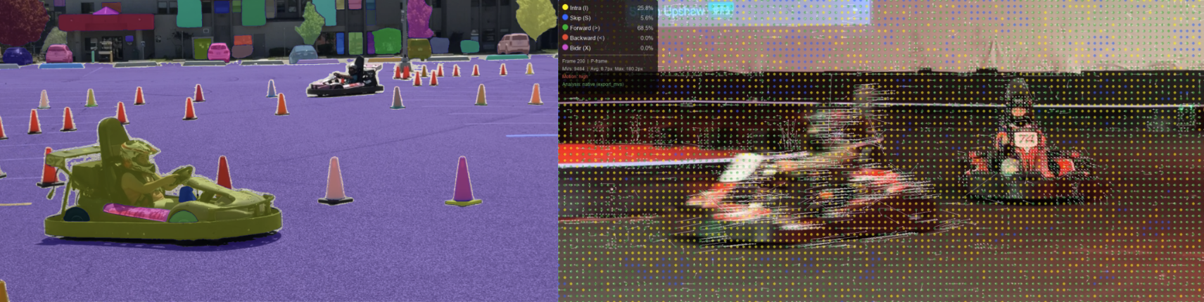
Motion Vectors in Video Compression
Video codecs exploit temporal redundancy: instead of encoding each frame from scratch, they find where blocks moved from the previous frame and encode only the difference.
Reference Frame
Current Frame
Motion Vector Field
Predicted Frame (from ref + MVs)
Residual (×4 amplified)
How it works: For each block in the current frame, the encoder searches the reference frame
for the best matching block (using Sum of Absolute Differences). The displacement is stored as a
motion vector (dx, dy). The predicted frame is assembled by copying
reference blocks according to these vectors. Only the small residual (current − predicted)
needs to be encoded, saving significant data. Areas with uniform motion (like camera pans) compress
especially well because many blocks share similar vectors.
Quantization Step-by-Step
Watch how DCT coefficients get divided and rounded for a single 8×8 block.
50
DCT Coefficients
÷
Quantization Matrix
=
Quantized (Rounded)
How the DCT Transforms a Block
See exactly how the Discrete Cosine Transform converts an 8×8 pixel block from spatial values
into frequency coefficients, and how each coefficient contributes to the reconstruction.
Input Pixels (click to edit)
⟶ DCT
DCT Coefficients
⟶ IDCT
Reconstructed Pixels
Input Block
Coefficient Magnitudes
Reconstructed
Partial Reconstruction
Progressive Reconstruction
Control how many DCT coefficients are included (in zigzag order, low→high frequency).
Watch the block build up from coarse to fine detail.
Zigzag Scan Order
Key insight: The DCT is lossless — with all 64 coefficients the block reconstructs
perfectly. Compression comes from discarding small high-frequency coefficients
(bottom-right in the matrix). The first coefficient (top-left, the DC term) captures
the average brightness. Each additional coefficient adds finer detail.
The zigzag scan orders coefficients from lowest to highest frequency so that
trailing zeros can be efficiently encoded.
Quantization creates long runs of zeros in the zigzag-scanned coefficients. Run-length encoding (RLE)
exploits these runs to dramatically reduce the data size. Compare the streams before and after quantization.
50
Before Quantization (Raw DCT Coefficients)
Zigzag-scanned stream:
As RLE tokens:
After Quantization (Q = 50)
Zigzag-scanned stream:
As RLE tokens:
Compression Comparison
DCT Coefficients (zigzag order overlay)
After Quantization
How RLE works in JPEG: After quantization, the 8×8 block is read in
zigzag order (low → high frequency). Each non-zero value is stored as
a pair: (run_of_zeros, value). When the remaining coefficients are all zero,
a special EOB (End of Block) symbol is emitted. Aggressive quantization creates
more zeros and earlier EOBs, yielding smaller output.
DCT Basis Functions
Each position in the 8×8 matrix corresponds to a 2D cosine wave pattern. Hover to see details.
Hover over a basis function to see its frequency description.
Position (0,0) is the DC component (average brightness). Moving right
increases horizontal frequency; moving down increases vertical frequency. The quantization matrix assigns
larger divisors to higher frequencies because the human visual system is less sensitive to fine detail.